Fogpy usage in a nutshell¶

The package uses OOP extensively, to allow higher level metaobject handling.

For this tutorial, we will use a MSG scene for creating different fog products.

Import satellite data first¶

We start with the PyTroll package satpy. This package provide all functionalities to import and calibrate a MSG scene from HRIT files. Therefore you should make sure that mpop is properly configured and all environment variables like PPP_CONFIG_DIR are set and the HRIT files are in the given search path. For more guidance look up in the `satpy`_ documentation

Note

Make sure satpy is correctly configured!

Ok, let’s get it on:

>>> from satpy import Scene
>>> from glob import glob
>>> filenames = glob("/path/to/seviri/H-000*20131212000*")
>>> msg_scene = Scene(reader="seviri_l1b_hrit", filenames=filenames)
>>> msg_scene.load([10.8])
>>> msg_scene.load(["fog"])

We imported a MSG scene from 12. December 2013 and loaded the 10.8 µm channel and the built-in simple fog composite into the scene object.

Now we want to look at the IR 10.8 channel:

>>> msg_scene.show(10.8)

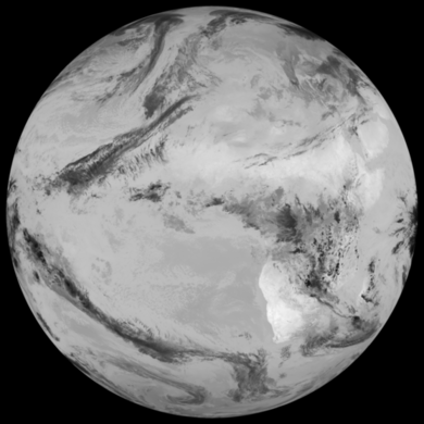
Everything seems correctly imported. We see a full disk image. So lets see if we can resample it to a central European region:

>>> eu_scene = msg_scene.resample("eurol")
>>> eu_scene.show(10.8)

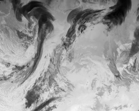
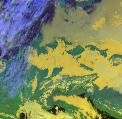
A lot of clouds are present over central Europe. Let’s test a fog RGB composite to find some low clouds:

>>> eu_scene.show("fog")

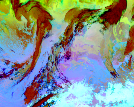
The reddish and dark colored clouds represent cold and high altitude clouds, whereas the yellow-greenish color over central and eastern Europe is an indication for low clouds and fog.

Continue with more metadata¶

In the next step we want to create a fog and low stratus (FLS) composite for the imported scene. For this we need:

Seviri L1B data, read by Satpy with the seviri_l1b_hrit reader.

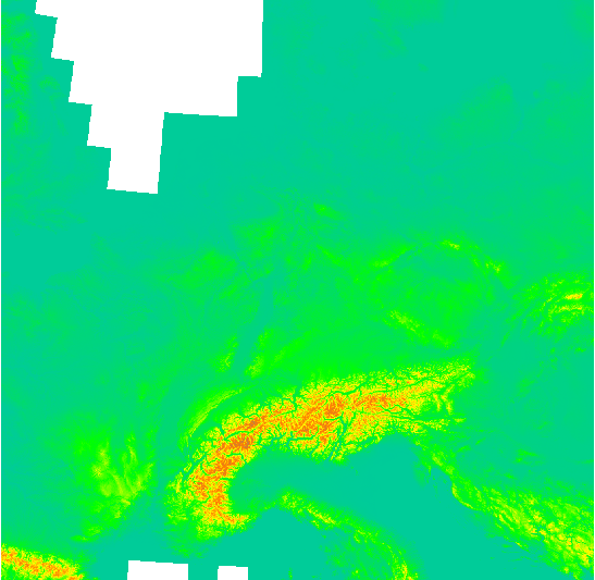
Cloud microphysical data, read by Satpy with the nwcsaf-geo reader. In principle, CMSAF data could also be used, but as of May 2019, there is no CM-SAF reader within Satpy.

A digital elevation model. This can derived from data available from the European Environmental Agency (EEA). Although this can be read by Satpy using the generic_image reader, the Fogpy composite reads this as a static image. The path to this image needs to be defined in the Fogpy etc/composites/seviri.yaml file.

We create a scene in which we load datasets using both the seviri_l1b_hrit and nwcsaf-geo readers. Here we choose to load all required channels and datasets explicitly:

>>> fn_nwcsaf = glob("/media/nas/x21308/scratch/NWCSAF/*100000Z.nc")
>>> fn_sev = glob("/media/nas/x21308/scratch/SEVIRI/*201904151000*")
>>> sc = Scene(filenames={"seviri_l1b_hrit": fn_sev, "nwcsaf-geo": fn_nwcsaf})
>>> sc.load(["cmic_reff", "IR_108", "IR_087", "cmic_cot", "IR_016", "VIS006",
             "IR_120", "VIS008", "cmic_lwp", "IR_039"])

We can now visualise any of those datasets using the regular pytroll visualisation toolkit. Let’s first resample the scene again:

>>> ls = sc.resample("eurol")

And then inspect the cloud optical thickness product:

>>> from trollimage.xrimage import XRImage
>>> from trollimage.colormap import set3
>>> xrim = XRImage(ls["cmic_cot"])
>>> set3.set_range(0, 100)
>>> xrim.palettize(set3)
>>> xrim.show()

Get hands-on fogpy at daytime¶

After we imported all required metadata we can continue with a fogpy composite.

Note

Make sure that the PPP_CONFIG_DIR includes fogpy/etc/ directory!

Fogpy comes with its own etc/composites/seviri.yaml. By setting PPP_CONFIG_DIR=/path/to/fogpy/etc, Satpy will find the fogpy composites and all fogpy composites can be used directly in Satpy.

Let’s try it with the fls_day composite. This composite determines low clouds and ground fog cells from a satellite scene. It is limited to daytime because it requires channels in the visible spectrum to be successfully applicable. We create a fogpy composite for the resampled MSG scene:

>>> ls.load(["fls_day"])

This may take a while to complete. You see that we don’t have to import the fogpy package manually. It’s done automagically in the background after the satpy configuration.

The fls_day composite function calculates a new dataset, that is now available like any other Satpy dataset, such as by ls["fls_day"] or ls.show("fls_day"). The dataset has two bands:

Band L is an image of a selected channel (Default is the 10.8 IR channel) where only the detected ground fog cells are displayed
Band A is an image for the fog mask

The result image shows the area with potential ground fog calculated by the algorithm, fine. But the remaining areas are missing… maybe a different visualization could be helpful. We can improve the image output by colorize the fog mask and blending it over an overview composite using trollimage:

>>> ov = satpy.writers.get_enhanced_image(ls["overview"]).convert("RGBA")
>>> A = ls["fls_day"].sel(bands="A")
>>> Ap = (1-A).where(1-A==0, 0.5)
>>> im = XRImage(Ap)
>>> im.stretch()
>>> im.colorize(fogcol)
>>> RGBA = xr.concat([im.data, Ap], dim="bands")
>>> blend = ov.blend(XRImage(RGBA))

Note

Images not yet updated!

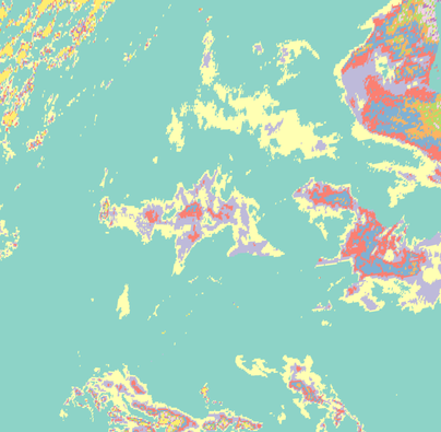
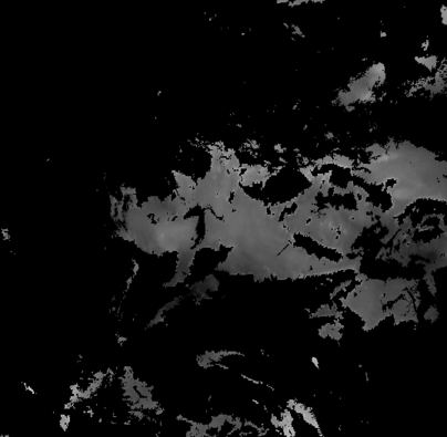
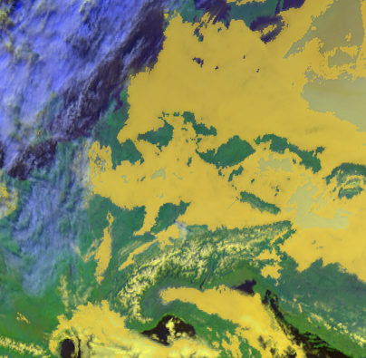
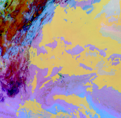
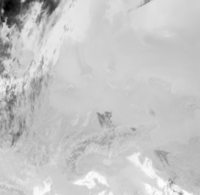
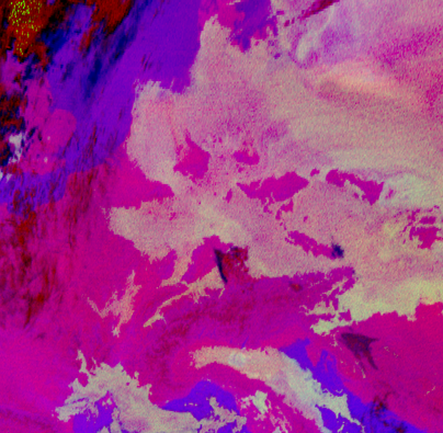
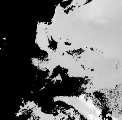
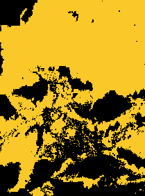
Here are some example algorithm results for the given MSG scene. As described above, the different masks are blendes over the overview RGB composite in yellow, except the right image where the fog RGB is in the background:


Cloud mask	Low cloud mask	Low cloud mask + Fog RGB

It looks like the cloud mask works correctly, except of some missclassified snow pixels in the Alps. But this is not a problem due to the snow filter which successfully masked them out later in the algorithm. Interestingly low cloud areas that are found by the algorithm fit quite good to the fog RGB yellowish areas.

On a foggy night …¶

We saw how daytime fog detection can be realized with the fogpy fls_day composite. But mostly fog occuring during nighttime. So let’s continue with another composite for nighttime fog detection fls_night:.

Note

Again make sure that the fogpy composites are made available in satpy!

First we need the nighttime MSG scene:

>>> fn_nwcsaf = glob("/media/nas/x21308/scratch/NWCSAF/*100000Z.nc") # FIXME: UPDATE!
>>> fn_sev = glob("/media/nas/x21308/scratch/SEVIRI/*201904151000*") # FIXME: UPDATE!
>>> sc = Scene(filenames={"seviri_l1b_hrit": fn_sev, "nwcsaf-geo": fn_nwcsaf})
>>> sc.load(["IR_108, "IR_039", "night_fog"])

Reproject it to the central European section from above and have a look at the infrared channel:

>>> ls = sc.resample("eurol")
>>> ls.show(10.8)

We took the same day (12. December 2017) as above. Now we could check whether the low clouds, that are present at 10 am, already can be seen early in the the morning (4 am) before sun rise.

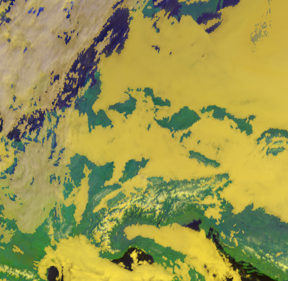
So let’s look at the nighttime fog RGB product:

>>> ls.show("night_fog")

As we see, a lot of greenish-yellow colored pixels are present in the night scene. This is a clear indication for low clouds and fog. In addition these areas have a similar form and distribution as the low clouds in the daytime scene. We can conclude that these low clouds should have formed during the night.

So let’s create the fogpy nighttime composite. Fogpy will use the PyTroll package pyorbital for solar zenith angle calculations, so make sure this one is installed. The nightime composite for the resampled MSG scene is generated in the same way like the daytime composite with `satpy`_:

>>> ls.load(["fls_night"])
>>> ls.show("fls_night")

It seems, the detected low cloud cells in the composite overestimate the presence of low clouds, if we compare the RGB product to it. In general, the nighttime algorithm exhibit higher uncertainty for the detection of low clouds than the daytime approach. Therefore a comparison with weather station data could be useful.

Gimme some ground truth!¶

Fogpy features some additional utilities for validation and comparison attempts. This include methods to plot weather station data from Bufr files over the FLS image results. The Bufr data is thereby processed by the trollbufr PyTroll package and the images are generated with trollimage. Here we load visibility data from German weather stations for the nighttime scene:

>>> import os
>>> from fogpy.utils import add_synop
    # Define search path for bufr file
>>> bufr_dir = '/path/to/bufr/file/'
>>> nbufr_file = "result_{}_synop.bufr".format(ntime.strftime("%Y%m%d%H%M"))
>>> inbufrn = os.path.join(bufr_dir, nbufr_file)
    # Create station image
>>> station_nimg = add_synop.add_to_image(nfls_img, tiffarea, ntime, inbufrn, ptsize=4)
>>> station_nimg.show()

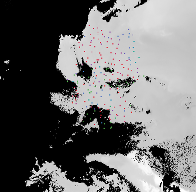
The red dots represent fog reports with visibilities below 1000 meters (compare with legend), whereas green dots show high visibility situations at ground level. We see that low clouds, classified by the nighttime algorithm not always correspond to ground fog. Here the station data is a useful addition to distinguish between ground fog and low stratus.

At daytime we can make the same comparison with station data:

>>> bufr_file = "result_{}_synop.bufr".format(time.strftime("%Y%m%d%H%M"))
>>> inbufr = os.path.join(bufr_dir, bufr_file)
    # Create station image
>>> station_img = add_synop.add_to_image(fls_img, tiffarea, time, inbufr, ptsize=4)
>>> station_img.show()

We see that the low cloud area in Northern Germany has not been classified as ground fog by the algorithm, whereas the southern part fits quite good to the station data. Furthermore some mountain stations within the area of the ground fog mask exhibit high visibilities. This difference is induced by the averaged evelation from the DEM, the deviated lower cloud height and the real altitude of the station which could lie above the expected cloud top. In addition the low cloud top height assignment can exhibit uncertainty in cases where a elevation based height assignment is not possible and a fixed temperature gradient approach is applied. These missclassifications could be improved by using ground station visibility data as algorithm input. The usage of station data as additional filter could refine the ground fog mask.

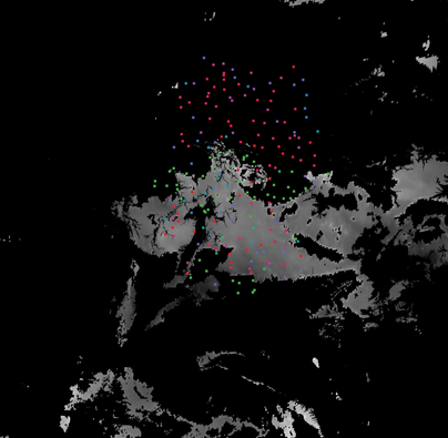
Luckily we can use the StationFusionFilter class from fogpy to combine the satellite mask with ground station visibility data. We use several dataset that had been calculated through out the tour as filter input and plot the filter result:

>>> from fogpy.filters import StationFusionFilter
    # Define filter input
>>> flsoutmask = np.array(fogmask.channels[0], dtype=bool)
>>> filterinput = {'ir108': dem_scene[10.8].data,
>>>                'ir039': dem_scene[3.9].data,
>>>                'lowcloudmask': flsoutask,
>>>                'elev': elevation.image_data,
>>>                'bufrfile': inbufr,
>>>                'time': time,
>>>                'area': tiffarea}
    # Create fusion filter
>>> stationfilter = StationFusionFilter(dem_scene[10.8].data, **filterinput)
>>> stationfilter.apply()
>>> stationfilter.plot_filter()

The data fusion revise the low cloud clusters in Northern Germany and East Europe as ground fog again. The filter uses ground station data to correct false classification and add missing ground fog cases by utilising a DEM based interpolation. Furthermore cases under high clouds are also extrapolated by elevation information. This cloud lead to low cloud confidence levels. For example the fog mask over France and England. The applicatin of this filter should be limited to a region for which station data is available to achieve a high qualitiy data fusion product. In this case the area should be cropped to Germany, which can be done by setting the limit attribute to True:

>>> filterinput['limit'] = True
    # Create fusion filter with limited region
>>> stationfilter = StationFusionFilter(dem_scene[10.8].data, **filterinput)
>>> stationfilter.apply()
>>> stationfilter.plot_filter()

The output is now limited automagically to the area for which station data is available.

The above station fusion filter example can be used to code any other filter application in fogpy. The command sequence more or less looks like the same:

Prepare filter input

Instantiate filter class object

Run the filter

Enjoy the results

All available filters are listed in the chapter Filters in fogpy. Whereas the algorithms that can be directly applied to PyTroll Scene objects can be found in the Algorithms in fogpy section.